 ช้างเผือก
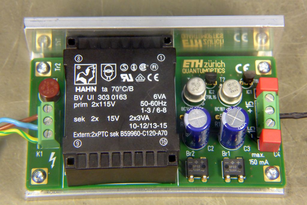
Categories
Statistics
Since 08.08.2014
Counts only, if "DNT = disabled".
216.73.216.253
216.73.216.253
Counts only, if "DNT = disabled".
216.73.216.253
216.73.216.253
Info

เราจะทำแบบวิศวกรผู้ยิ่งใหญ่

27. July 2026
YOUR OPINION •••
average: 0.001, n: 0

When using this form, your ip is stored in order to avoid multiple voting on the same website. That's it.
When using this form, your ip is stored in order to avoid multiple voting on the same website. That's it.
PowerSupplyCharacterisation.php 15619 Bytes 04-03-2025 19:13:22
Power Supply Characterisation
Test Procedures for Power Supplies
You just built your own Power Supply. Great ! But how good is it really ?
 Tinkering around with the Powerline is dangerous. Advanced users only. An
isolation transformer or FI-switch is mandatory. Even Professionals use that kind of gear !
Tinkering around with the Powerline is dangerous. Advanced users only. An
isolation transformer or FI-switch is mandatory. Even Professionals use that kind of gear !
✈ Stages of Tests
We divided this overview in three timezones of a running Power Supply.
| TIMEZONE | WHAT TO LOOK AT |
| 1 | Power On 1: Time to reach Specifications 2: Warm-Up Drift |
| 2 | En Route 1: Drift 2: Ripple + Noise = PARD (periodic and random deviation) 3: Efficiency 4: Stability : Line Regulation 5: Load Regulation : Output Impedance and Load Transient Response 6: Overload Conditions - Current Limiting |
| 3 | Long Term Behaviour 1: Stability - Long Term Drift 2: Ageing |
1.1: Time to reach Specifications
The time used to warm up the device to a thermal equilibrum and the output to reach its
specified stability. This usually is in the range of minutes up to hours. The manufacturer (you)
does specify that timespan.
Even so the supply is capable of working immediately after it is turned on, it is necessary
to allow this time, when powering sensitive devices.
1.2: Warm-Up Drift
This figure quantifies the change in Output Voltage during Warm-Up. You need
to take two measurements of the Output Voltage under its rated full load.
The first measurement is taken 10 - 20 seconds after power-on. The second
measurement is taken, after the Power Supply has reached its thermal equilibrium.
If you don't have a value to hand, measure after 60 minutes. With those two
values, we mayst calculate the Drift in percent.

The time it takes to stabilise is influenced by the circuit design, the thermal mass and the way the air is guided thru the case.
The time it takes to stabilise is influenced by the circuit design, the thermal mass and the way the air is guided thru the case.
2.1: Drift
This figure is meaning almost the same as the above. The only difference is, that it is measured
after a warm-up period. Other influences like Line-Voltage or Temperature are kept constant.
You just define a timespan (e.g. 8 hrs, 1000 hrs) in which the wandering of the output voltage is observed.
Wandering means anything below 20 Hz. Very useful are Voltmeters, which can store minimum and maximum values.
2.2: Ripple + Noise = PARD (periodic and random deviation)
These are two ac components which sit on the dc component. The term 'Ripple' is used to describe
voltage variations coming from the (bridge) rectifier. It usually has a frequency of n * 50 Hz.
The most dominant part is likely to be 100 Hz. Noise is everything else. In order to have a meaningful
value, the measurement bandwidth needs to be specified. A common value is 20 MHz.
The Ripple can be expressed by :

The noise can be expressed by an integration over the measurement bandwidth. We prefer a plot of the spectrum, as a picture says more than 1000 words ...
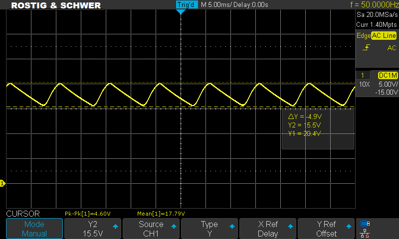
DC Output of 17.8 V and the superimposed PARD (periodic and random deviation) of 4.6 Vpp
The noise can be expressed by an integration over the measurement bandwidth. We prefer a plot of the spectrum, as a picture says more than 1000 words ...
DC Output of 17.8 V and the superimposed PARD (periodic and random deviation) of 4.6 Vpp
2.3: Efficiency
It is widely known, that switching power supplies are more efficient than linear regulators.
You made that topology decision already. Even so you mayst own your own power plant,
the Efficiency Graph may point you to design errors or weaknesses.
And if not, you have your first characteristic value. Ideally this value is 100%,
but in real world, you are "in business" with 90% - 95% (when using a switching regulator).
For this measurement, you need 4 multimeters Two times in Voltage mode, two times in current mode and a big load resistor (or an electronic load). Whilst some decades ago, people discussed the exact position of those multimeters, they have become that good nowadays, that such discussions have only theoretical value.
You need to measure the Power going into the supply, that mayst be : Vac and Iac and the Power coming out which is very likely Vdc and Idc. The Efficiency is then calculated as follows :
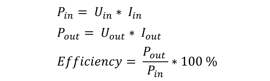
And yes : the Output Power is always smaller than the Input Power. If that's not the case, double check your measurements.
For this measurement, you need 4 multimeters Two times in Voltage mode, two times in current mode and a big load resistor (or an electronic load). Whilst some decades ago, people discussed the exact position of those multimeters, they have become that good nowadays, that such discussions have only theoretical value.
You need to measure the Power going into the supply, that mayst be : Vac and Iac and the Power coming out which is very likely Vdc and Idc. The Efficiency is then calculated as follows :
And yes : the Output Power is always smaller than the Input Power. If that's not the case, double check your measurements.
2.4: Stability : Line Regulation
The Voltage of the Powerline is never constant. Nor is its Frequency.
This 230 V thing is a nominal value. It could in the very worst case fluctuate by ± 20 %.
The Stability or Stabilization Factor describes, how a Power Supply suffers from such changes.
For this measurement, you need a Transformer with a variable output.
The absolute Stabilization Factor is the Ratio of the Input Voltage Change versus the Output Voltage Change. Measured under nominal Load conditions. The input voltage is changed by e.g. ± 10 %. The larger this value is, the better the regulation in the Power Supply works.
The absolute Stabilization Factor G (sometimes also called Smoothingfactor) and the relative Stabilization Factor S are calculated as follows :
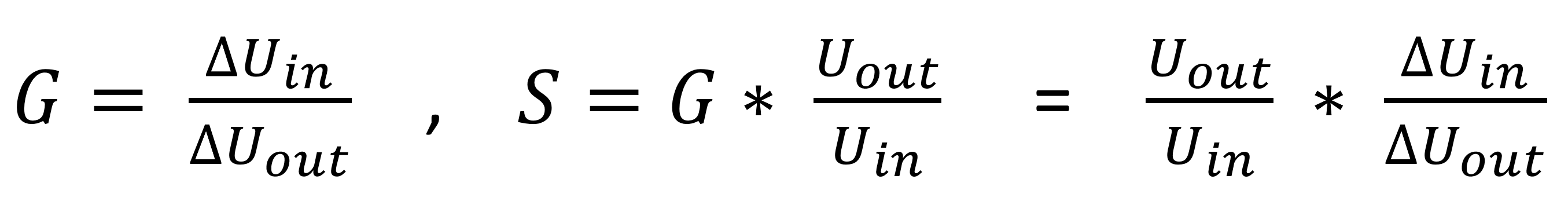
It is not mandatory to change the input voltage by exactly ± 10 %. Sometimes this value is too large. You just have to note the values at which you measured them. The user of your device must be able to reproduce that measurement.
The absolute Stabilization Factor is the Ratio of the Input Voltage Change versus the Output Voltage Change. Measured under nominal Load conditions. The input voltage is changed by e.g. ± 10 %. The larger this value is, the better the regulation in the Power Supply works.
The absolute Stabilization Factor G (sometimes also called Smoothingfactor) and the relative Stabilization Factor S are calculated as follows :
It is not mandatory to change the input voltage by exactly ± 10 %. Sometimes this value is too large. You just have to note the values at which you measured them. The user of your device must be able to reproduce that measurement.
2.5: Stability : Load Regulation (slow and fast)
The Load of a Power Supply may also vary. Slowly or fast. To cover the slow change,
the Output Impedance is used, whilst for fast changes, the Load Transient Response
is helpful.
The Output Impedance can be measured with two different load conditions. This yields in two Voltages and two Currents. The Output Impedance then can be calculated as :

The Load Transient Response is a dynamical (fast) test. It can be done with every better electronic load. If you don't have such exclusive equipment, a big resistor and a switching transistor will also work fine. Select the switching transistor therefore, that it can be switched on by a TTL signal at the gate. A setup may look like this :
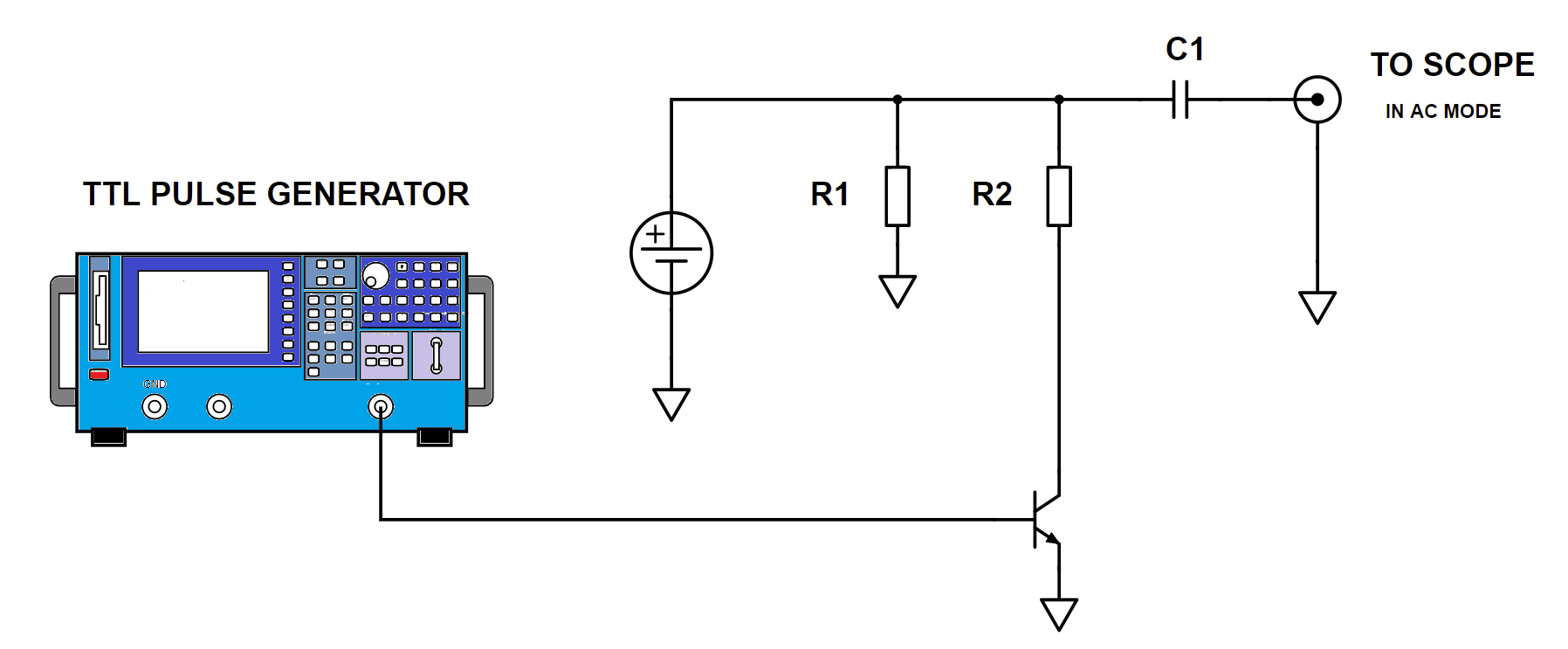
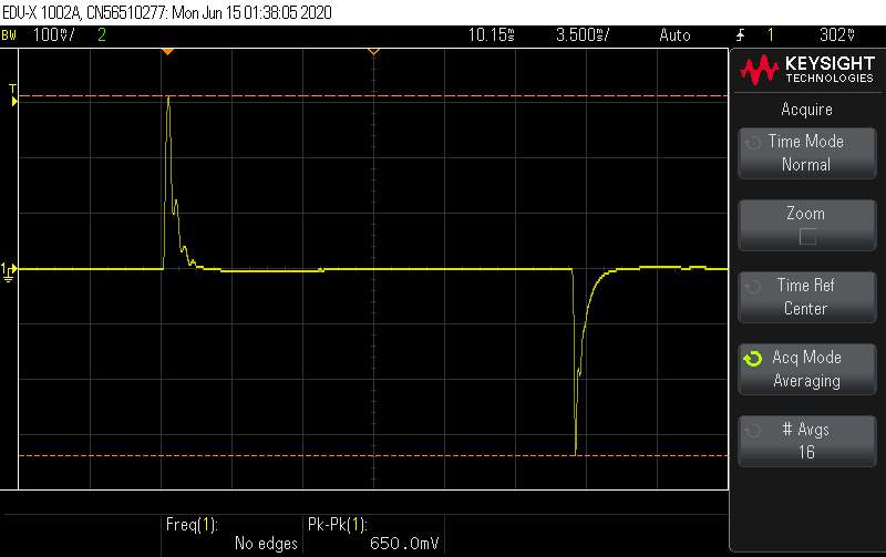
R1 is used to load the Power Supply by e.g. 10%, R2 loads for an additional 80%. When switching R2 on and off, the overall load changes from 10% to 90% - and back. On the Scope you can monitor the step response. This gives you valuable information on the speed of the regulation and much more. The Supplymod showed the following behaviour :
The Output Impedance can be measured with two different load conditions. This yields in two Voltages and two Currents. The Output Impedance then can be calculated as :
The Load Transient Response is a dynamical (fast) test. It can be done with every better electronic load. If you don't have such exclusive equipment, a big resistor and a switching transistor will also work fine. Select the switching transistor therefore, that it can be switched on by a TTL signal at the gate. A setup may look like this :
R1 is used to load the Power Supply by e.g. 10%, R2 loads for an additional 80%. When switching R2 on and off, the overall load changes from 10% to 90% - and back. On the Scope you can monitor the step response. This gives you valuable information on the speed of the regulation and much more. The Supplymod showed the following behaviour :
2.6: Overload Conditions - Current Limiting
When powering new or unknown circuits for the first time, a current limit function
is often useful. As a maximum current at a given voltage creates heat, which must be
dissipated, there are different strategies to deal with that.
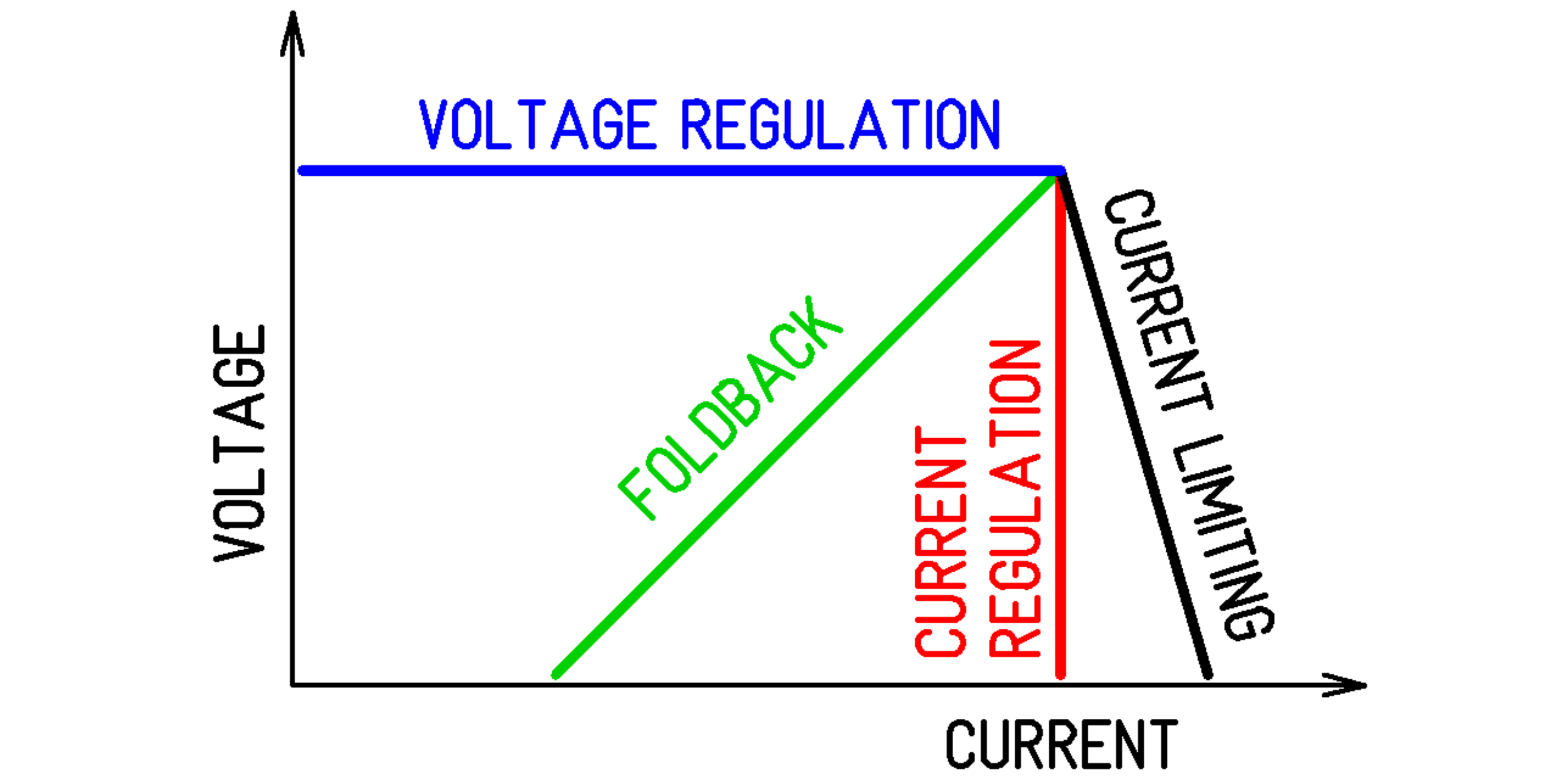
The ideal (best) case is, when the voltage is constant until the current limit is reached and the power supply then holds the current constant. (blue + red). This is also the most challenging (expensive) design. Very often, the current is limited, but not that constant. (blue + black). And the poorest combination is the blue and green behavior. Here the current drops to a very low level, once it exceeded the maximum treshhold. I stays there forever - no attempt to go back into the voltage regulation mode is made, even if the load has changed.
Very high quality power supplies (blue + red) can withstand a short at the output for an infinite time, as the heatsink is hopelessly oversized. The second category (blue + black) can endure an overload condition for a certain amount of time - until a thermal fuse kicks in and shuts down the supply. (This may recover when cooled down). And the third combination (blue + green) can withstand a short at the output for an infinite time, as the dissipated power is very low - and therefore the (small) heatsink is not overstrained.
3.1: Stability - Long Term Drift
This is very similiar to the other drifts, mentionned above. Except, that the timescale
has been increased by some decades. You'll usually find such information only at very high
quality gear.
3.2: Ageing
Ageing describes the change of properties with time under the influence of heat.
Like with humans, a faster ageing leads to an earlier death. Speaking in terms
of electronics, this means a higher temperature during operation. That's why
high reliable equipment uses bigger heatsinks - to get the temperature down. It is
clear, that such measures are more expensive.
The life expectation of a device is inverse proportional to the integral of the temperature versus time.
In order to characterise the ageing bahaviour, there are two possible methods. First, operate the device for a long time and observe it. Secondly, observe the device under stressful conditions like heat and observe it. As time to market is usually a criteria, the industry uses climat chambers to force the ageing process.
4: Appendix

✈ Share your thoughts
The webmaster does not read these comments regularely. Urgent questions should be send via email.
Ads or links to completely uncorrelated things will be removed.
|
t1 = 7319 d
t2 = 441 ms |
★ ★ ★ Copyright © 2006 - 2026 by changpuak.ch ★ ★ ★
|
|